
Is the market bluffing when option prices imply far more future swing than history shows?
Historical volatility measures what already happened, while implied volatility is the market’s forward-looking guess baked into option prices.
For traders, that gap changes pricing, risk sizing, and which strategies make sense.
This post breaks the math into plain terms, explains why the IV-HV gap matters, and lists the watch items: earnings, liquidity, and vega exposure, so you can trade with clearer odds.
Core Differences Between Implied and Historical Volatility Explained

Historical volatility tells you what already happened. Implied volatility shows what the market thinks will happen. That’s the simple version, but the practical consequences for traders touch everything from pricing to risk management to which strategy you pick.
Historical volatility is just the standard deviation of past returns over whatever window you choose. Could be 10 days, 30, or 90. Then you annualize it by multiplying by the square root of 252, which is roughly how many U.S. trading days you get in a year. The calculation uses actual price changes, usually daily log returns, to build a backward looking measure. If a stock shows 25 percent annualized historical volatility over the last 30 days, that number describes how much the price bounced around during that stretch. It doesn’t predict anything. It summarizes.
Implied volatility comes from option prices, backed out using a pricing model. Black–Scholes is the most common, sometimes paired with a numerical solver like Newton–Raphson. It’s the market’s collective guess about future volatility, baked into the premium traders pay or collect for options. When the market prices an option at 40 percent implied volatility, that reflects how much uncertainty traders are hedging or betting on. Implied volatility looks forward and reacts to supply, demand, events, and sentiment shifts.
Here’s a quick example. If 30 day historical volatility sits at 25 percent and implied volatility on near dated options is 40 percent, the market is pricing way more expected uncertainty than recent experience shows. The options cost more than the realized moves would justify based on history alone.
The most important splits are:
Data inputs: historical volatility uses realized price returns. Implied volatility uses current option prices.
Forecasting use: historical volatility gives you a baseline from the past. Implied volatility embeds forward expectations and risk premium.
Pricing impact: implied volatility directly sets option premiums. Historical volatility doesn’t appear in any option quote.
Stability: historical volatility changes gradually as new returns replace old ones. Implied volatility can spike or collapse within hours around news.
Interpretation: historical volatility quantifies what you observed. Implied volatility quantifies what the market is willing to pay to hedge or bet on.
Historical Volatility Calculation and Interpretation

Calculating historical volatility starts with a series of daily price returns. Traders like log returns, computed as the natural log of today’s close divided by yesterday’s. Log returns add nicely across time and approximate percentage changes for small moves. Once you’ve got a series for, say, the past 30 trading days, you compute the sample standard deviation of those 30 numbers. That’s your daily volatility figure. To annualize it, multiply by the square root of 252, the typical number of trading days in a year. The result is annualized historical volatility as a percentage. 30 day historical volatility came in at 28 percent annualized, which means the daily standard deviation scaled to a full year.
The lookback window you pick affects sensitivity and noise. A 10 day window captures very recent moves and reacts fast to sudden price changes, but it can be noisy and unstable. A 90 day or 180 day window smooths volatility across market regimes and is less prone to whipsaw, but it lags recent shifts. Traders often watch multiple windows at once to tell short term spikes from structural changes. If 20 day historical volatility is 35 percent but 90 day is 22 percent, something unusual happened recently.
Historical volatility also depends on measurement frequency. Daily returns are standard, but intraday or weekly returns produce different numbers even for the same period. The annualization factor has to match. Daily returns use sqrt(252), weekly returns use sqrt(52), and so on. Historical volatility clusters too. High volatility tends to follow high volatility, and low follows low, a pattern that simple standard deviation doesn’t model. Recognize that historical volatility is a descriptive statistic, not a forecast, and it depends on regime, window, and calculation method.
| Window (days) | Typical Use | Notes |
|---|---|---|
| 10–20 | Short-term tactical signals | Reacts quickly, can be noisy, good for event-driven moves |
| 30–60 | Medium-term context | Balances recency and stability, common benchmark for options comparisons |
| 90–180 | Long-term baseline | Smooths regimes, less reactive, used for risk budgeting and position sizing |
| 250 | Full-year trailing volatility | Captures annual cycles, useful for VaR and multi-period models |
How Implied Volatility Is Derived from Option Prices

Implied volatility gets pulled from option prices by inverting a pricing model. In Black–Scholes, you input the current stock price, strike, time to expiration, risk free rate, and the observed market price of the option. The only unknown is volatility. Solving for the volatility that makes the model output match the market price gives you implied volatility. Since Black–Scholes has no closed form solution for volatility, traders use numerical root finding techniques, usually Newton–Raphson, which iterates toward the implied volatility that zeroes the gap between model price and market price. The algorithm adjusts the vol guess until the model spits out the exact premium you see quoted.
Vega measures how much an option’s price changes for a one percentage point change in implied volatility. If an option has a Vega of 0.20, a one point rise in implied volatility bumps the option price by roughly $0.20, all else equal. Vega is highest for at the money options and longer dated expirations. Vega exposure matters because implied volatility can shift suddenly, especially around earnings, Fed meetings, or geopolitical events. A trader long options is long Vega, benefiting when implied volatility rises. A seller of options is short Vega and profits when implied volatility falls or stays low.
Liquidity and market structure affect implied volatility readings. Wide bid ask spreads, low open interest, or stale quotes can distort the derived implied volatility. Thin markets produce unreliable implied volatility, and event driven spikes can make IV jump well above any historical baseline without reflecting a true change in expected realized volatility. Just a scramble for protection.
Bid ask spreads: wide spreads inflate implied volatility calculated from mid prices. Always check volume before trusting IV.
Low open interest: illiquid strikes often show elevated or erratic IV. These readings are noise, not signals.
Implied surface discontinuities: gaps or jumps in the volatility surface across strikes or expirations point to pricing inconsistencies or stale data.
Event driven spikes: earnings, FDA decisions, or elections can push implied volatility far above historical norms temporarily. The spike fades post event.
Comparative View: Implied vs Historical Volatility in Practice

Placing implied volatility and historical volatility side by side shows their roles and limits in a trading workflow.
| Metric | Data Source | Direction (Lookback/Forward) | Use Case | Notes |
|---|---|---|---|---|
| Implied Volatility (IV) | Option market prices | Forward-looking | Option pricing, strategy selection, expected move | Includes risk premium; can spike on events; varies by strike and expiration |
| Historical Volatility (HV) | Realized price returns | Lookback | Risk assessment, stop-loss sizing, VaR, baseline comparison | Window-dependent; clusters; does not forecast; annualization via sqrt(252) |
| Realized Volatility | Actual price moves during option life | Post-facto outcome | P&L attribution, model validation, hedge performance | Knowable only after expiration; basis for comparing IV to outcome |
The gap between implied volatility and historical volatility often points to mispricing or shifts in market expectations. When implied volatility exceeds historical volatility by a wide margin, say IV at 40 percent versus 30 day HV at 25 percent, options are pricing higher future uncertainty than recent experience. This richness can create opportunities for premium sellers, who collect elevated premiums betting that realized volatility will fall short of implied. Flip it around. When implied volatility sits below historical volatility, options are relatively cheap, favoring buyers who expect a reversion or continuation of recent volatility. If HV has averaged 30 percent and IV is only 22 percent, long straddles or calendars may offer positive edge if realized volatility stays elevated.
Implied volatility also carries a volatility risk premium. That’s the extra cost investors pay to hedge tail risk and uncertainty. Over long periods, implied volatility tends to overstate realized volatility, compensating sellers for taking on jump risk and event uncertainty. This premium isn’t constant. It compresses in calm markets and expands during stress. Recognizing that implied volatility is not a pure forecast but a hedging cost helps traders avoid the mistake of treating IV as a prediction. Implied volatility is what you pay, realized volatility is what you get, and the difference is the risk premium plus forecast error.
Numerical Examples Comparing IV and HV

Consider a stock trading at $50 with 30 day historical volatility of 25 percent annualized. At the money options expiring in 30 days show an implied volatility of 40 percent. The 15 point difference (40 minus 25 equals 15 percentage points) signals that the market is pricing significantly more expected movement than the stock exhibited recently. For a trader, this gap suggests options are expensive relative to the recent baseline. A premium seller might look to short straddles or credit spreads, betting that realized volatility over the next 30 days will be closer to the historical 25 percent than the implied 40 percent. You’re collecting 40 percent premium to hedge 25 percent moves. That’s a positive edge if the pattern holds.
In a second scenario, the same $50 stock shows 30 day historical volatility of 35 percent but near dated implied volatility of only 28 percent. Options are cheaper than recent experience suggests. A volatility buyer might purchase a straddle or calendar spread, expecting realized volatility to stay elevated or rebound. If realized volatility remains near 35 percent, the long option position benefits from Vega gains as implied volatility reprices higher or from intrinsic value accumulation as the stock moves. When IV undershoots HV and the stock is choppy, long premium can capture both Vega expansion and directional swings.
Vega helps quantify the sensitivity. Suppose an at the money call with 30 days to expiration has a Vega of 0.18. If implied volatility rises from 28 percent to 33 percent, a five point jump, the option price gains roughly 0.18 times 5 equals $0.90, all else equal. For a trader long 10 contracts, that’s a $900 gain from the Vega component alone. Flip it. A seller with the same position loses $900 if implied volatility jumps. Vega exposure scales with position size and time to expiration, making it a critical input for risk management. Short premium during low IV sounds appealing until an event spike doubles your Vega loss overnight.
Divergences worth watching include:
IV well above recent HV: options are expensive. Favor premium selling, credit spreads, covered calls if you believe realized won’t justify the price.
IV below recent HV: options are cheap. Favor buying straddles, long calendars, or protective puts if you expect continued or elevated realized volatility.
IV spike with stable HV: often event driven, like earnings or a data release. Post event IV typically collapses quickly.
HV spike with lagging IV: can indicate mispriced options or delayed market reaction. Opportunity for volatility buyers before IV catches up.
Trading Applications Using Implied and Historical Volatility

Implied volatility drives option pricing and strategy selection. When setting up a trade, a trader compares implied volatility to a forecast or historical baseline to decide whether to buy or sell premium. High implied volatility makes options expensive, tilting the edge toward sellers who collect rich premiums and hope realized volatility disappoints. Low implied volatility makes options cheap, tilting toward buyers who expect a volatility pickup. This comparison is the foundation of volatility trading. You’re not betting on direction. You’re betting on whether the market’s priced in uncertainty is too high or too low relative to what will actually happen.
Historical volatility serves risk management and position sizing. A trader uses historical volatility to estimate stop loss thresholds, value at risk, and margin requirements. If 30 day historical volatility is 20 percent, a one standard deviation daily move is roughly 20 divided by sqrt(252), about 1.26 percent. For a $100 stock, that’s a $1.26 expected daily swing. Setting a stop loss two standard deviations away, about $2.50, gives room for normal noise while protecting against adverse moves. Historical volatility also informs position sizing. Higher volatility assets get smaller position sizes to keep portfolio risk constant. If stock A has twice the HV of stock B, you hold half the notional to equalize volatility contribution.
Volatility skew and smile affect strike selection within a strategy. Skew refers to the variation in implied volatility across strikes for the same expiration. In equity markets, out of the money puts typically carry higher implied volatility than at the money or out of the money calls, reflecting demand for downside protection. A volatility smile is a U shaped pattern where both wings, deep in the money and out of the money, show elevated IV relative to at the money. Traders exploit skew by selling rich wings and buying cheaper strikes, or by using vertical spreads that benefit from relative IV mispricing. If OTM puts are trading 45 percent IV and ATM is 35 percent, selling a put spread captures that 10 point skew premium.
Volatility Skew and Smile in Strategy Selection
Skew and smile shape the payoff and risk profile of multi leg strategies. A trader constructing an iron condor sells both an out of the money call spread and an out of the money put spread. If the put side has 10 points more implied volatility than the call side, the put spread collects more premium for the same width, skewing the risk reward asymmetrically. Recognizing this skew, the trader might widen the call spread or narrow the put spread to balance credit and probability. Calendar spreads also depend on the volatility term structure. If near term IV is elevated relative to longer dated IV, selling the front month and buying the back month can profit from time decay and mean reversion in the front month IV. You’re betting the spike in front month IV collapses faster than the back month IV, pocketing the difference.
Workflow: Combining Implied and Historical Volatility for Decisions
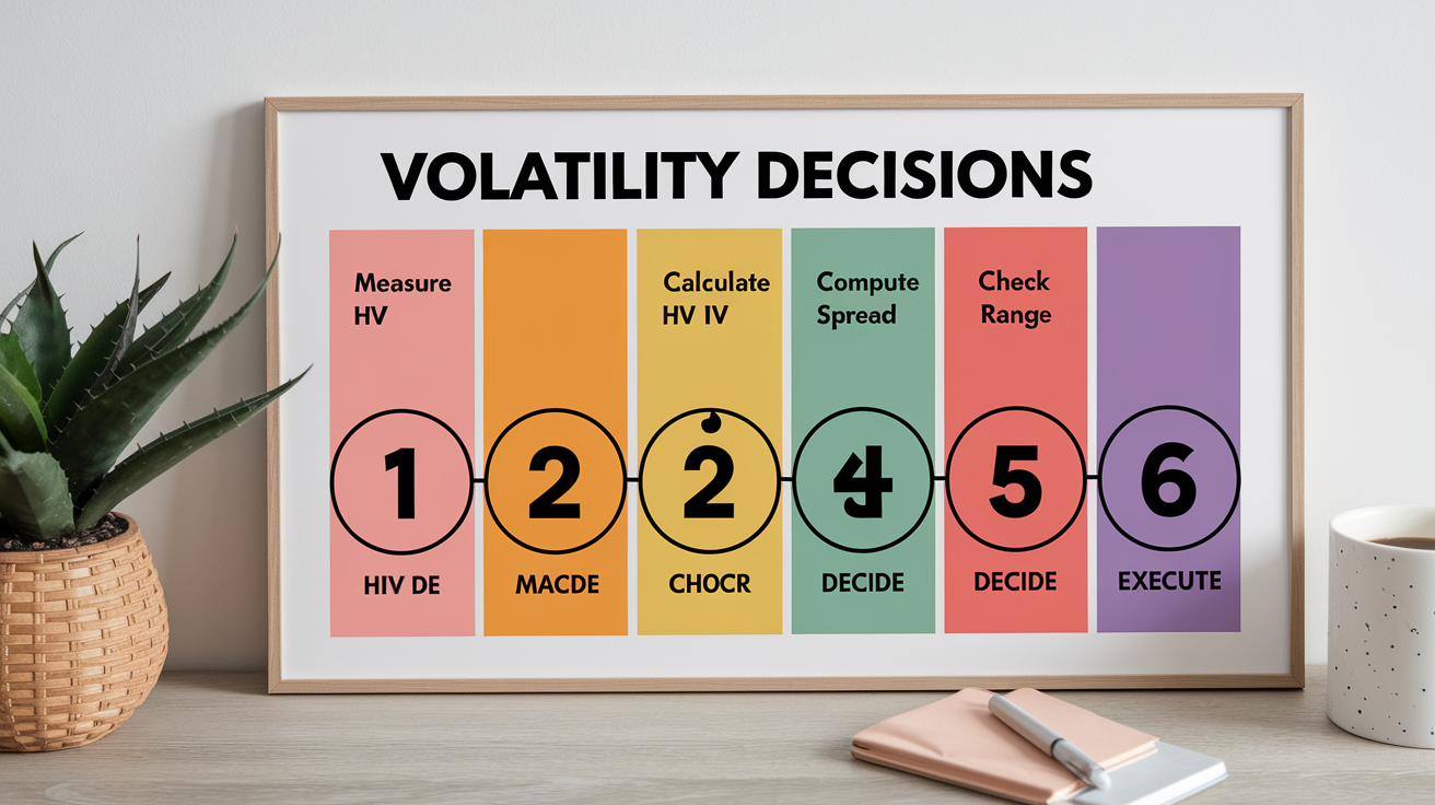
A structured workflow helps traders move from observation to action using both implied and historical volatility. The process starts with measurement and comparison, then interprets the divergence, and finally selects strategies aligned with the signal.
Start by ensuring apples to apples comparison. Use the same annualization method and similar time horizons. If you’re evaluating 30 day options, compare implied volatility to 30 day historical volatility, both annualized. Mixing a 10 day HV with 60 day IV creates false signals. Tools and platforms often display multiple historical volatility windows. Choose the one closest to your option’s time to expiration. Match the lookback to the forward look. If your options expire in 45 days, use 45 day historical volatility as the baseline.
The six step decision checklist is:
- Measure current implied volatility from the options chain for the expiration and strikes you’re considering.
- Calculate historical volatility for a window matching the option’s life. For example, 30 day HV for 30 day options.
- Compute the IV–HV spread: subtract HV from IV to see if options are rich (positive spread) or cheap (negative spread).
- Check the historical range: compare today’s IV to its own 52 week percentile. If IV is at the 90th percentile, it’s expensive by recent standards even if HV is elevated.
- Incorporate risk premium and regime: remember IV typically includes a premium. During calm regimes, expect IV to exceed realized by a few points. During stress, gaps widen.
- Select strategy based on the signal: IV significantly above HV and at high percentile favors selling premium. IV below HV or at low percentile favors buying premium or hedging with options.
Limitations and Caveats of IV and HV

Implied volatility is not a forecast. It’s a market derived expectation that embeds hedging demand, sentiment, and risk premium. Traders sometimes mistake high implied volatility for a prediction of large moves, but IV often overstates realized volatility because it includes compensation for tail risk and uncertainty. Post event, implied volatility frequently collapses regardless of the actual move size. Earnings IV can be 60 percent before the announcement and drop to 30 percent the next day, even if the stock moved 10 percent. The event premium evaporated, not the realized volatility.
Historical volatility depends on window length, return definition, and market regime. A 10 day window captures only the most recent moves and can spike or crash quickly. A 250 day window smooths across an entire year but may mix multiple regimes, low volatility trending markets and high volatility drawdowns, into one average that obscures recent shifts. The choice of log returns versus simple returns also affects the number, though the difference is usually small for daily calculations. Historical volatility clusters, meaning high volatility begets high volatility, so a single spike can elevate HV for the entire lookback window. One gap down day can inflate 20 day HV for weeks until it rolls out of the sample.
Low liquidity options distort implied volatility severely. Wide bid ask spreads, infrequent trades, and stale quotes produce unreliable IV readings. Around major events like earnings, FDA rulings, or elections, implied volatility spikes due to demand for hedges, not because realized volatility is expected to stay elevated indefinitely. The event premium typically vanishes within hours after the announcement, leaving sellers who collected the spike with quick profits and buyers with collapsing premiums. Don’t mistake event driven IV for structural volatility. It’s a one time insurance premium, not a forecast of sustained choppiness.
FAQs About Implied and Historical Volatility

What is the difference between realized volatility and historical volatility? Realized volatility is the actual standard deviation of returns measured over a completed period. Historical volatility is the same concept applied to any past window, typically reported before the option expires. Both are backward looking, but “realized” often refers to the specific period an option was live.
How is implied volatility surface constructed? The implied volatility surface is a three dimensional plot showing IV across strike prices and expirations. Traders fit models, local volatility or stochastic volatility, to observed option prices to interpolate and smooth IV for strikes and dates not actively traded.
Why do longer dated options often show different implied volatility than near term options? The volatility term structure reflects different expectations and risk premiums across horizons. Near term IV can spike on imminent events while longer dated IV stays stable, or mean reversion expectations can invert the term structure during calm periods.
How does annualization work, and why sqrt(252)? Volatility scales with the square root of time under the assumption that returns are independent. 252 is the approximate number of U.S. trading days per year, so multiplying daily standard deviation by sqrt(252) converts it to an annualized figure comparable across assets and periods.
Final Words
We showed that historical volatility measures past price swings while implied volatility reflects the market’s expectation priced into options. That backward-looking versus forward-looking split is the core difference.
Use HV to size risk and set stop thresholds; use IV to price trades, pick strategies, and spot when sellers demand a premium. Skew and liquidity matter too.
Watch divergences and term structure rather than guessing which is “right.” Treat implied volatility vs historical volatility as complementary tools, and your decisions will be clearer.
FAQ
Q: What does 20% implied volatility mean?
A: The 20% implied volatility means the market is pricing about a 20% annualized standard deviation for the underlying, implying roughly a ±20% one‑sigma move over the next year under current expectations.
Q: What is the difference between IV and HV?
A: The difference between IV and HV is IV is the market’s forward‑looking volatility implied by option prices (often with a risk premium), while HV is the backward‑looking standard deviation of past returns over a chosen window.
Q: Is 30% IV high?
A: A 30% IV is moderately high for many equities; whether it’s high depends on the asset, its typical HV, sector peers, and upcoming events—compare IV to historical norms to judge relative richness.
Q: How much IV is good for options?
A: How much IV is good for options depends on your strategy: buyers prefer lower current IV that can rise later, sellers like higher IV to collect richer premiums; always compare IV to HV and your time horizon.